Shift Invariance Experiments

See our Paper Website!

Description

tl;dr provided below

Modern convolutional neural networks for object image classification have been shown to be very sensitive to the location of the object in the image. This may be due to biases in the training data or the architecture of the model itself. In this experiment, we evaluate such sensitivity by exhaustively shifting an object in an image and comparing features extracted from hidden layers and target class probabilities.

Datasets

We generated datasets by shifting a transparent patch across a background image, or by cropping a patch from a larger image. The currently available datasets are:

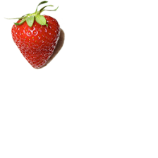
• berry: A 100x100 transparent image of a strawberry was shifted with stride 1 across a 224x224 completely white background. Its target class in ILSVRC2012 is 949: 'strawberry'.
• plane: A 224x224 image was cropped from a 356x356 image of a military jet with stride 1. Its target class in ILSVRC2012 is 895: 'warplane, military plane'.

Models

We evaluate pretrained models provided by torchvision [link] and pretrained antialiased models provided with "Making Convolutional Networks Shift-Invariant Again" by Richard Zhang, published in ICML 2019 [link]. Details regarding training are:

• torchvision: Models were trained on ILSVRC2012. Data was augmented with random resized cropping [docs] and random horizontal flipping. The training script is available [here].
• antialiased: Models were trained on ILSVRC2012. Architectures were directly modified from the torchvision models. Data was agumented with random resized cropping [docs] and random horizontal flipping. Training information is available [here].

Models and Layers

The following models and layers are currently available:

• Alexnet
  • fc6: The first fully connected layer, before ReLU.
  • fc6relu: The fc6 layer after the ReLU activation function.
  • fc7: The penultimate fully connected layer, before ReLU.
  • fc7relu: The fc7 layer after the ReLU activation function.
  • fc: The final fully connected layer, before softmax.
  • class: Target class probability.
• VGG16
  • fc6: The first fully connected layer, before ReLU.
  • fc6relu: The fc6 layer after the ReLU activation function.
  • fc7: The penultimate fully connected layer, before ReLU.
  • fc7relu: The fc7 layer after the ReLU activation function.
  • fc: The final fully connected layer, before softmax.
  • class: Target class probability.
• Resnet50
  • fc: The final fully connected layer, before softmax.
  • class: Target class probability.
• MobileNetV2
  • fc: The final fully connected layer, before softmax.
  • class: Target class probability.

Method

For each image in each dataset, we extract hidden layer activations (currently, only fully connected layers) as 1-dimensional feature vectors. Then, after selecting an anchor feature, we calculate the cosine similarity between it and all other features. These values are plotted as a heatmap in 2 dimensions (each axis representing the object shifting in each dimension). A fully shift-invariant network would have features that do not change depending on object location (a cosine similarity of 1 across the heatmap).
For each image in each dataset, we also retrieve the confidence of the corresponding target class. These values are not comparative, and are simply plotted on the heatmap. These values are represented as the "class" layer.

Results

The tool below allows for interactive browsing of the results. Different models, layers, and datasets can be selected with the dropdown menus. For features extracted from hidden layers, the feature to calculate the cosine similarity against (the "Anchor Image") can also be selected.
The two heatmaps for each model/layer/dataset/anchor combination is plotted below. The heatmap on the left shows results from the torchvision model, and the heatmap on the right shows results from the antialiased model. Sliders on the bottom can change the minimum value for the colormap (the maximum value is fixed at 1.0). Finally, hovering over the plot shows the corresponding image and value on the left panel.

tl;dr

Convolutional neural networks can classify images as different objects, but they break if you move the image around a little. Pick a popular classification model that people use as benchmarks in the top left dropdown. Pick betwen a strawberry and a plane in the top middle dropdown. Ignore the top right dropdown. Select the "class" layer on the bottom left dropdown. Hover over the left or right heatmap to move the object, and see how the model's confidence that the object is a berry or plane changes from 0 to 1 (Try ResNet50 & plane). Use the slider at the bottom to change the range of the heatmap color. The model of the left heatmap is inconsistent at recognizing moved objects but it's the one everyone uses. The model of the right heatmap improves the consistency with antialiasing. Please read the paper for full details and context.

cosine similarity =
1.0

(simulated with css)